RobMixReg: an R package for robust, flexible and high dimensional mixture regression – Supplementary Materials
Wennan Chang
Hanming Ye
Changlin Wan
Chun Yu
Weixin Yao
Chi Zhang
Sha Cao
Source:vignettes/tutorial.Rmd
tutorial.RmdS1. Introduction
Regression-based association analysis remains to be the most popular data mining tool for hypothesis generation, owing to its ease of inter-pretability. However, the traditional linear regression model cannot adequately fit the complexity of the biomedical data caused by: 1) high leverage noise and outliers resulted from the large scale technical experiments; 2) the presence of subpopulations among the wide spectrum of collected samples; 3) the high-dimensionality of the molecular features. Finite Mixture Gaussian Regression (FMGR) is a widely used model to explore the latent relationship between the response and predictors, and the goal of mixture regresison is to maximize the following likelihood: \[ argmax \sum_{i=1}^N log(\sum_{k=1}^K \pi_k \phi(y_i - \mathbf{x}_i^T \mathbf{\beta}_k ; 0, \sigma_k^2 )) \] Here, we are modeling the relationship between \(\mathbf{x}\) and \(y\) as a mixture of \(K\) regression lines, \(K \geq 1\). \((\mathbf{x_i}, y_i)\) is the \(i\)-th observations \(i=1,...,N\), \(\mathbf{\beta}_k\) are the regression coefficients for the \(k\)-th regression line; \(\epsilon_{ik}\) is the error term; \(\sigma_k\) is the standard deviation of \(\epsilon_{ik}\).
‘RobMixReg’ is a package that provides a comprehensive solution to mining the latent relationships in biomedical data, ranging from the regulatory relationships between different molecular elements, to the the relationships between pheno-types and omic features, in the presence of outliers, latent subgroups and high dimensional molecular features.
The major contribution of RobMixReg lies in the following key aspects: 1) for low dimensional predictors, it handles outliers in modeling the latent relationships, and provides flexible modeling to allow for different predictors for different mixture components; 2) for high dimensional predictors, it detects subgroups and select informative features simultaneously. The RobMixReg package is a powerful exploratory tool to mining the latent relationships in data, which is often obfuscated by high leverage outliers, distinct subgroups and high dimensional features.
The RobMixReg package could be installed from CRAN:
It could be also installed from GitHub:
#library("devtools")
#devtools::install_github("changwn/RobMixReg")
S2. Case Studies
S2.0 Data Simulation:
The function simu_func is used to generate the synthetic data for various of cases. The input of simu_func is :
\(\beta\) A matrix whose \(k\)-th column is the regression coefficients matrix for the \(k\)-th component
\(\sigma\) A vector whose \(k\)-th element is the standard deviation of the error term for the \(k\)-th regression component
alpha The proportion of the observations being contaminated by the outlier
The output of simu_func is :
\(x\) Matrix of the predictors with dimension \(N \times (P+1)\), where \(P\) is the total number of predictors, and the first column is an all-one vector.
\(y\) Vector of response variable where alpha proportion of the observations are contaminated by outliers.
S2.1 Robust mixture regression
We adopt the mean-shift model in the presence of outliers, such that each outlier requires one additional parameter to cancel out the unusually large residuals. The outlier parameters are then regularized to achieve a balance of model complexity and model fitness.
\[ argmax \sum_{i=1}^N log(\sum_{k=1}^K \pi_k \phi(y_i - \mathbf{x}_i^T \mathbf{\beta}_k - \gamma_{ik} \sigma_k ; 0, \sigma_k^2 )) - \sum_{i=1}^N \sum_{k=1}^K P_{\lambda} (|\gamma_{ij}|) \]
Here, \(\gamma_{ik}\) models the level of outlierness for the \(i\)-th observation; \(P_{\lambda}(|\gamma_{ij}|)\) is a penalty function with a tuning parameter \(\lambda\) controlling the degrees of penalization on the \(\gamma_{ik}\).
We have intergrated multiple state-of-the-art methods in our package to robustly fit two or more regression lines. The default method is CAT. Other options inlcude TLE, flexmix, mixLp, mixbi, and they could be passsed to the MLM function by the parameter ‘rmr.method’. Among them, CAT and TLE could detect the identities of the outliers, and outliers are removed before model estimation; while the rest of the methods perform model estimation in the presence of outliers. For TLE to work, a trimming proportion needs to be provided, and the default is 0.05.
# simulate single variable x and y with linear relationship but contaminated by outliers.
set.seed(12345)
beta = rbind(c(0.2, 0.8), c(7, -0.6));  sigma=c(0.1,0.1); alpha=0.05;
data_case3 = simu_func(beta, sigma, alpha)
x3 = data_case3$x
y3 = data_case3$y
# Runing robust mixture regression by setting parameter 'ml.method'
# to 'rmr' in the wrapper function MLM.
res.c = MLM(ml.method="rmr", rmr.method='cat',x=x3, y=y3,nc=2) # CAT method
# Trimmed likelihod estimation. Here, the uers need to
# provide the ratio of outlier smaples.
res.c.TLE = MLM(ml.method="rmr", rmr.method='TLE', x=x3, y=y3)
res.c.flexmix = MLM(ml.method="rmr", rmr.method='flexmix', x=x3, y=y3)
res.c.Lp = MLM(ml.method="rmr", rmr.method='mixLp', x=x3, y=y3)
res.c.bi = MLM(ml.method="rmr", rmr.method='mixbi', x=x3, y=y3)
We can extract the outlier samples from the output of MLM.
## [1] 9 36 47 55 85 97 104 110 119 166 185 199 201 208 254 280
inds_in = which(res.c$cluMem != -1)The mixture regression parameters could be extracted by:
res.c$coff## Comp.1 Comp.2
## coef.(Intercept) 7.0315721 0.21468572
## coef.x -0.6076626 0.80190381
## sigma 0.0939840 0.09240652
## 0.5147829 0.48521712Here, the first two rows are regression coefficients, third row for the standard deviations, and fourth row for the component proportions.
We can visualize the fitted regression and the outliers by ‘compPlot’ function with ‘rlr’ parameter, shows in figure 1.
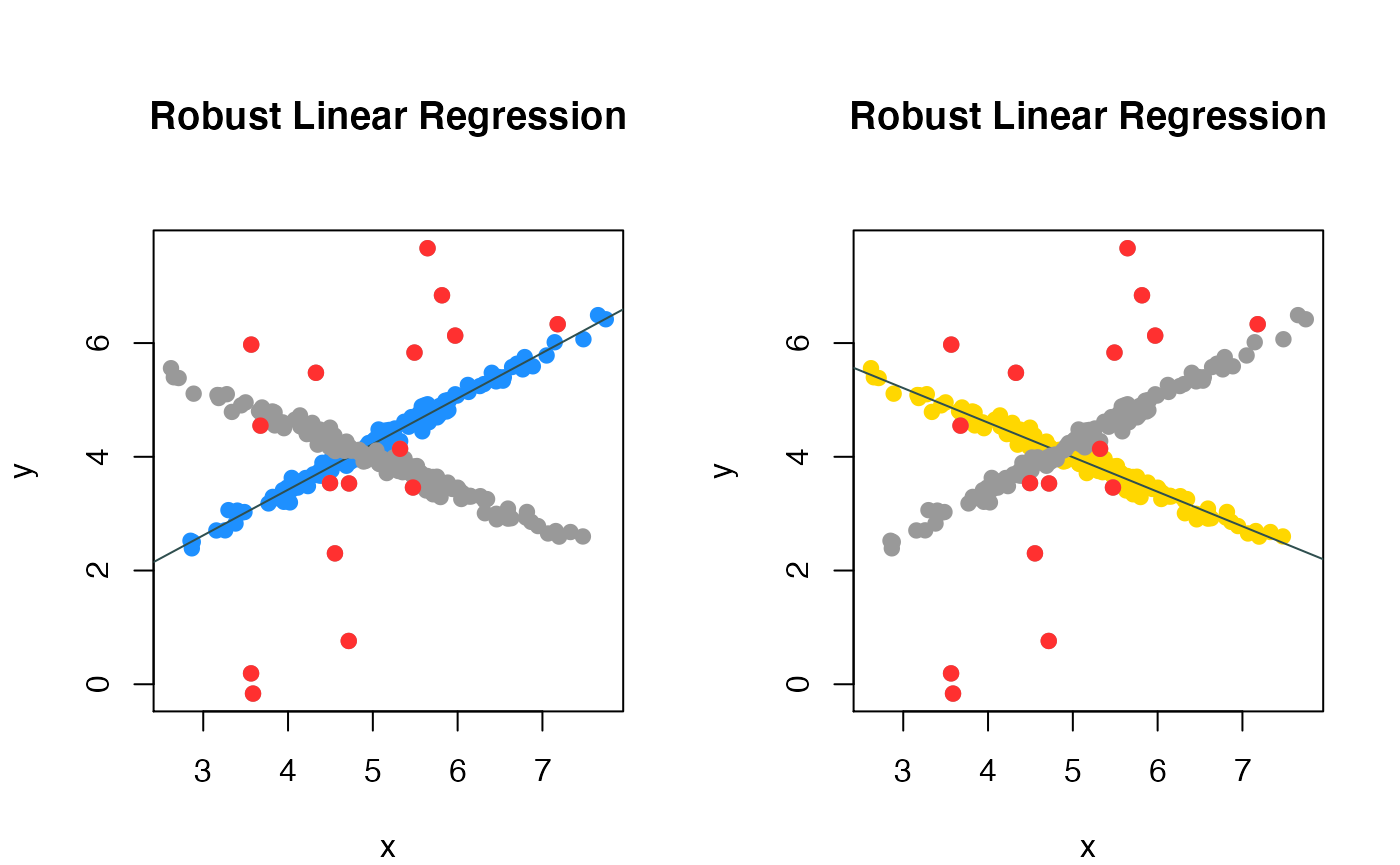
Robust mixture regression result
When \(K=1\), this degenerates to ordinary robust linear regression. We call for robust linear regression in the MLM wapper function by letting the ‘ml.method’ equal to ‘rlr’. In the core of the method is the ‘ltsReg’ function from the ‘robustbase’ package.
# Simulate single variable x and y with linear relationship but contaminated by outliers.
beta = c(1, 0.8); sigma=0.3; alpha= 0.1
data_case1 = simu_func(beta, sigma, alpha)
x1 = data_case1$x
y1 = data_case1$y
# Runing robust linear regression by setting parameter ml.method
# to 'rlr' in the wrapper function MLM.
res.a = MLM(ml.method='rlr', x=x1, y=y1)
We can extract the outlier samples from the output of MLM.
##  [1]  10  32  36  49  55  69  70  85 109 119 133 162 166 199 201 202 205 208 218
## [20] 234 261 290 299
The regression parameters could be extracted by:
res.a$coff## [,1]
## Intercept 0.9986726
## coef.x 0.8118485
## sd 0.2902440We can visualize the fitted regression and the outliers by compPlot function in figure 2.
inds_in = which(res.a$cluMem == 1)
# set the figure format and margin
par(mfrow=c(1,1),mar = c(5, 8, 2, 8))
# use plot module to draw the data points and the regression line.
compPlot(type='rlr', x=x1,y=y1,nc=1, inds_in=inds_in)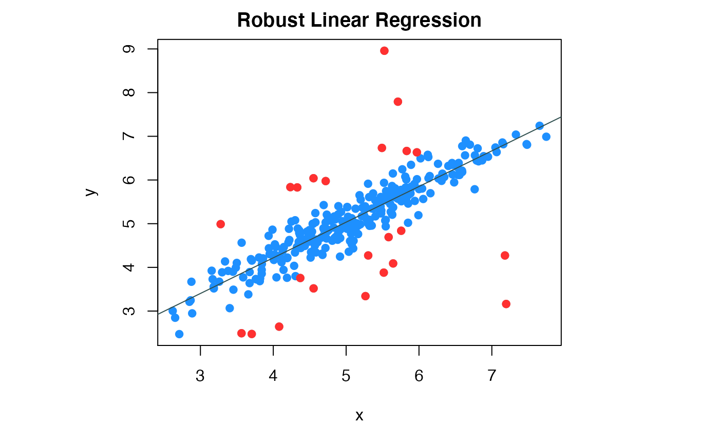
Robust linear regression result
S2.2 Mixture regression with flexible modeling
When fitting two or more lines through the data, there could be different regimes with the predictors in different lines. For example, two lines may involve different subsets of the predictors; or a line could include nonlinear transformations of the predictors to relax the “linearity” concerns. Different from the traditional mixture regression, RobMixReg allows for different set of predictors and their transformations as predictors for different component.
\[ argmax \sum_{i=1}^N log(\sum_{k=1}^K \pi_k \phi(y_i - g_k^T(\mathbf{x}_i) \mathbf{\beta}_k ; 0, \sigma_k^2 )) \]
Here, \(g_k(\cdot)\) is a vectorized function that transforms the original predictors in regression componetn \(K\), to combinations of the predictors and their transformations.
RobMixReg can easily achieve flexible modeling by specifying the regression formulas for different components. To enable flexible mixture regression, we call robust mixture regression in the MLM wapper function by letting the ‘ml.method’ be ‘fmr’. In the core of the method is the ‘mixtureReg’ function from the ‘mixtureReg’ package.
# simulate single variable x and y with linear relationship but contaminated by outliers.
# beta = c(0.8, -0.01); inter = c(0.2, 4)
beta = rbind(c(0.2, 0.8), c(4, -0.01)); sigma = c(1,1)
data_case2 = simu_func(beta, sigma,alpha=NULL)
x2 = data_case2$x
y2 = data_case2$y
# Runing robust mixture regression by setting parameter 'ml.method'
# to 'fmr' in the wrapper function MLM.
res.b = MLM(ml.method='fmr', x = x2, y = y2,
            b.formulaList = list(formula(y ~ x),formula(y ~ 1)))
The mixture regression parameters could be extracted by:
res.b$coff## 1 2
## Intercept 0.20084960 3.94766052
## coff.x 0.80273914 0.00000000
## sd 0.09104395 0.09222377
## mx 0.50333333 0.49666667Here, the first two rows are regression coefficients, third row for the standard deviations, and fourth row for the component proportions.
We can visualize the fitted regression lines by compPlot function and declare the ‘type’ parameter as ‘mr’ shows in figure 3.
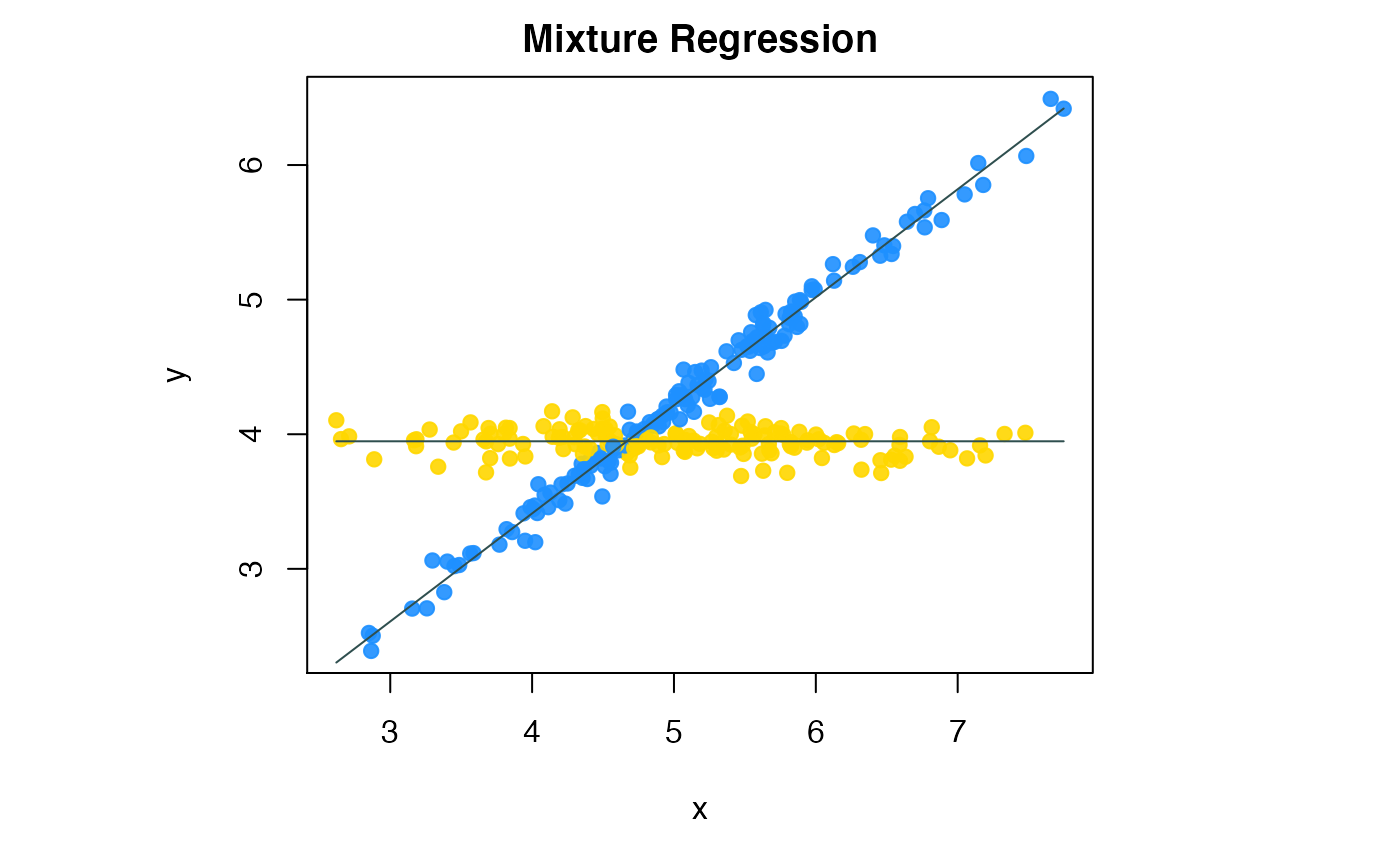
Flexible mixture regression result
S2.3 High dimensional mixture regression
Given high dimensional predictors, which is often the case in biological data, we have the total number of parameters to be estimated far more than the total number of observations, making the aofrementioned methods fail. In addition, the dense linear coefficients makes it hard to deduce the subgroup specific features and make meaningful interpreta-tions. We need to add regularization to the regression coefficients to achieve sparse mixture regression.
- Mathmatical Model
\[ argmax \sum_{i=1}^N log(\sum_{k=1}^K \pi_k \phi (y_i - \mathbf{x}_i^T \mathbf{\beta}_k ; 0,\sigma_k^2)) - \sum_{k=1}^K \lambda_k (\sum_{j=1}^P |\beta_{jk}|) \]
Different from the low dimensional setting, we are imposing constraints on the coefficients through the penalty parameter \(\lambda_k\). The CSMR algorithm is used here, which adaptively selects the penalty parameters \(\lambda_k\), hence there is no need for model selection with regards to \(\lambda_k\).
# simulate single variable x and y with linear relationship but contaminated by outliers.
set.seed(12345)
bet1=bet2=rep(0,101)
bet1[2:21]=sign(runif(20,-1,1))*runif(20,2,5)
bet2[22:41]=sign(runif(20,-1,1))*runif(20,2,5)
bet=rbind(bet1,bet2)
tmp_list = simu_func(beta=bet,sigma=c(1,1),alpha=NULL)
x=tmp_list$x
print(paste("Dimension of matrix (x):", dim(x)[1], ', ', dim(x)[2],sep='') )
## [1] "Dimension of matrix (x):400, 100"## [1] "Length of outcome variable (y):400"The mixture regression parameters could be extracted by:
head(res.d$coff)## 1 2
## feature1 0 3.272612
## feature2 0 2.918706
## feature3 0 5.028459
## feature4 0 4.107363
## feature5 0 -3.922227
## feature6 0 -3.189251Here, the first \((P+1)\) rows are regression coefficients, \((P+2)\)-th row for the standard deviations, and \((P+3)\)-th row for the component proportions.
We visualize the fitted coefficients using heatmap shows in figure 4. The columns are the clusters and the rows are the features.
#par(mfrow=c(1,1),mar = c(0.1, 0.1, 0.1, 0.1))
compPlot(type='block', res=res.d)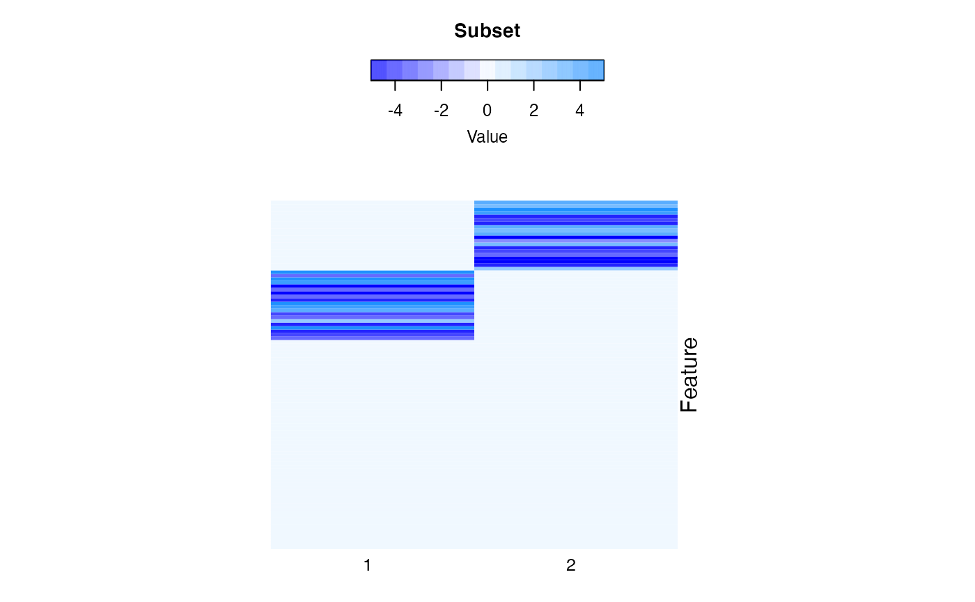
High dimensional feature space robust mixture regression result
S2.4 Order Selection
BIC based order selection
We provide two methods for selecting the number of components, \(K\): Bayesian information criterion (BIC) and cross validation. Meanwhile, in flexible modeling, even with the same \(K\), the models could still differ in their complexity, and we also provided BIC metric for model selection. The BIC of each fitted model could be extraced in slot ‘BIC’ by declaring the parameter ‘ml.method’:
Robust mixture regression using BIC
res.ba = MLM(ml.method='rlr', x=x1, y=y1)
res.bc = MLM(ml.method="rmr" ,x=x1, y=y1,nc=2)
res.bb = MLM(ml.method="rmr" ,x=x1, y=y1,nc=3)
print(res.ba$BIC)
## [1] 278.27
print(res.bc$BIC)## [1] 228.905
print(res.bb$BIC)## [1] 231.0611Flexbile mixture regression using BIC
res.fa = MLM(ml.method='fmr', x = x2, y = y2,
            b.formulaList = list(formula(y ~ x),formula(y ~ 1)))
res.fb = MLM(ml.method='fmr', x = x2, y = y2,
            b.formulaList = list(formula(y ~ x),formula(y ~ x)))
res.fc = MLM(ml.method='fmr', x = x2, y = y2,
            b.formulaList = list(formula(y ~ x),formula(y ~ x+ I(x^2))))
res.fd = MLM(ml.method='fmr', x = x2, y = y2,
            b.formulaList = list(formula(y ~ x),formula(y ~ x),formula(y ~ x)))

# res.b = MLM(ml.method='fmr', x = x2, y = y2,
#             b.formulaList = list(formula(y ~ x),formula(y ~ 1)))
print(res.fa$BIC)
## [1] 990.9967
print(res.fb$BIC)## [1] 1285.598
print(res.fc$BIC)## [1] 1585.6
print(res.fd$BIC)## [1] 2180.238High dimensional mixture regression using BIC
set.seed(111)
bet1=bet2=bet3=bet4=rep(0,81)
bet1[2:11]=sign(runif(10,-1,1))*runif(10,2,5)
bet2[12:21]=sign(runif(10,-1,1))*runif(10,2,5)
bet=rbind(bet1,bet2)
tmp_list = simu_func(beta=bet,n=200)
x=tmp_list$x
y=tmp_list$y
print(paste("Dimension of matrix (x):", dim(x)[1], ', ', dim(x)[2],sep='') )
## [1] "Dimension of matrix (x):200, 80"
hx=x;hy=y## [1] 5572.211Cross validation based order selection
For high dimensional predictors, we also provide cross validation for selection of \(K\).A large \(K\) will tend to overfit the data with more complex model of higher variance, while smaller \(K\) might select a simpler model with larger bias. Take a 5-fold cross validation as an example. For given \(K\), at each repetition, 80% samples are used for training to obtain the mixture regression parameters. Then, for any sample from the rest of the testing data, it is first assigned to a cluster by maximum posterior probability; then a prediction of \(\hat y\) could be made based on the model parameters given \(x\). Using the testing data, we could decide how to balance the trade-off between bias and variance. To evaluate how the estimated model under \(K\) explains the testing data, we could calculate the root-meansquare-error between the observed \(y\) and the predicted \(\hat y\), or Pearson correlation between the two. By repeating this procedure for multiple times, a more robust and stable evaluation of the choice of \(K\) should be derived based on the summarized RMSE or Pearson correlations.
The output of cross validation function, MLM_cv, is the average correlation or RMSE on the testing data. Higher correlation and lower RMSE indicate a better model with good bias variance tradeoff.
CV1 = MLM_cv(x=hx, y=hy, nc=2)## [1] "Fold 1 done."
## [1] "Fold 2 done."
## [1] "Fold 3 done."
## [1] "Fold 4 done."
## [1] "Fold 5 done."
print(CV1$ycor)## [1] 0.8613101
print(CV1$RMSE)## [1] 29.34191S3. Real Data Application
S3.1 Colon adenocarcinoma disease application
Colon adenocarcinoma is known as a heterogeneous disease with different molecular subtypes. We demonstrate the usage of oRobMixRegon collected expression of a few genes and the methylation profiles for some of their CpG sites from the Cancer Genome Atlas (TCGA) cohort.
data(colon_data)
x1 = colon_data$x1
y1 = colon_data$y1
res1 = MLM(ml.method='rlr', x=x1, y=y1)
inds_in = which(res1$cluMem == 1)
par(mfrow=c(1,1),mar = c(5, 8, 2, 8))
compPlot(type='rlr', x=x1,y=y1,nc=1, inds_in=inds_in)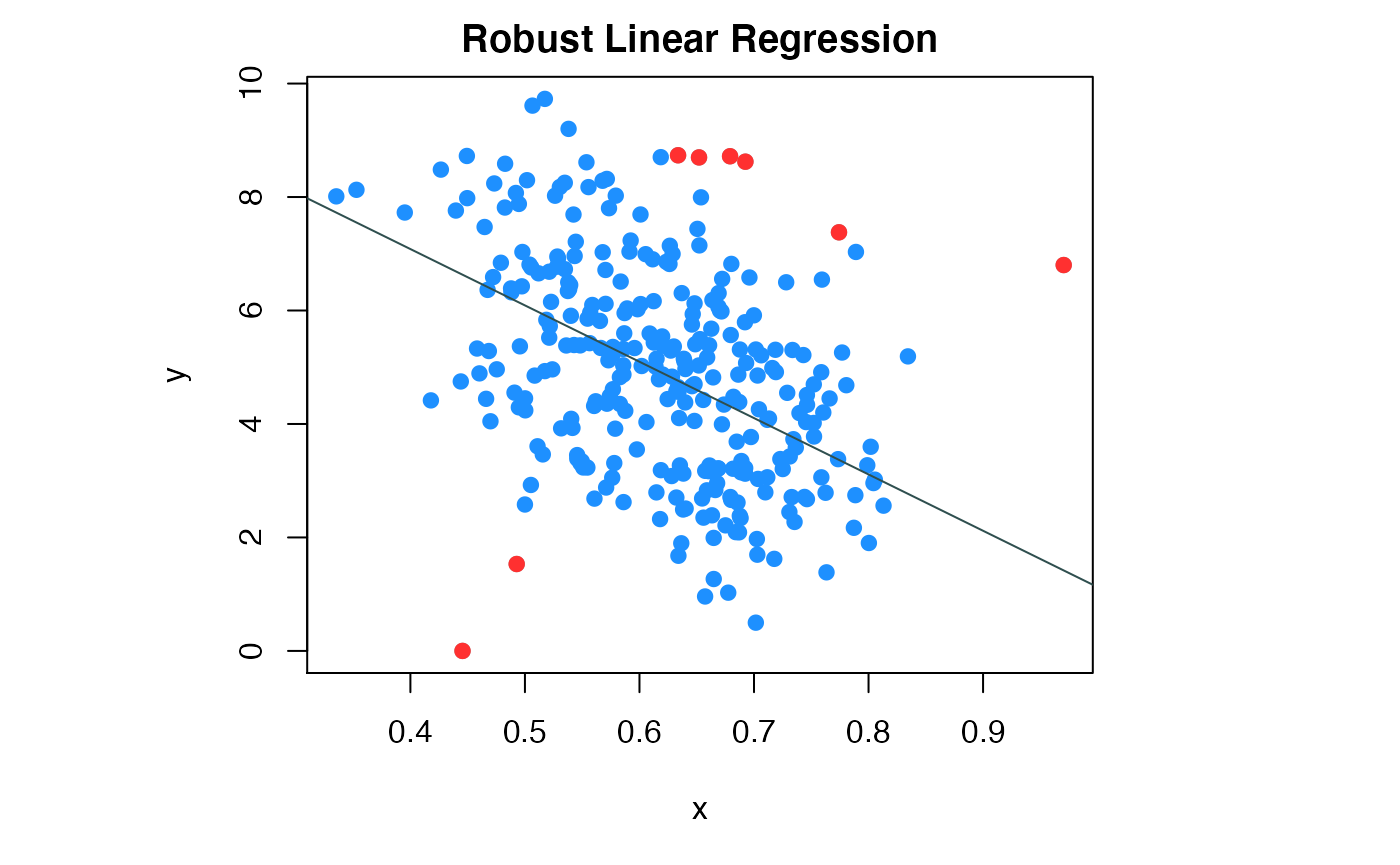
Colon data robust linear regression
data(colon_data)
x2 = colon_data$x2
y2 = colon_data$y2
res.b = MLM(ml.method='fmr', x = x2, y = y2,
            b.formulaList = list(formula(y ~ x),formula(y ~ 1)))
par(mar = c(5, 8, 2, 8))
compPlot(type='mr', res=res.b$res)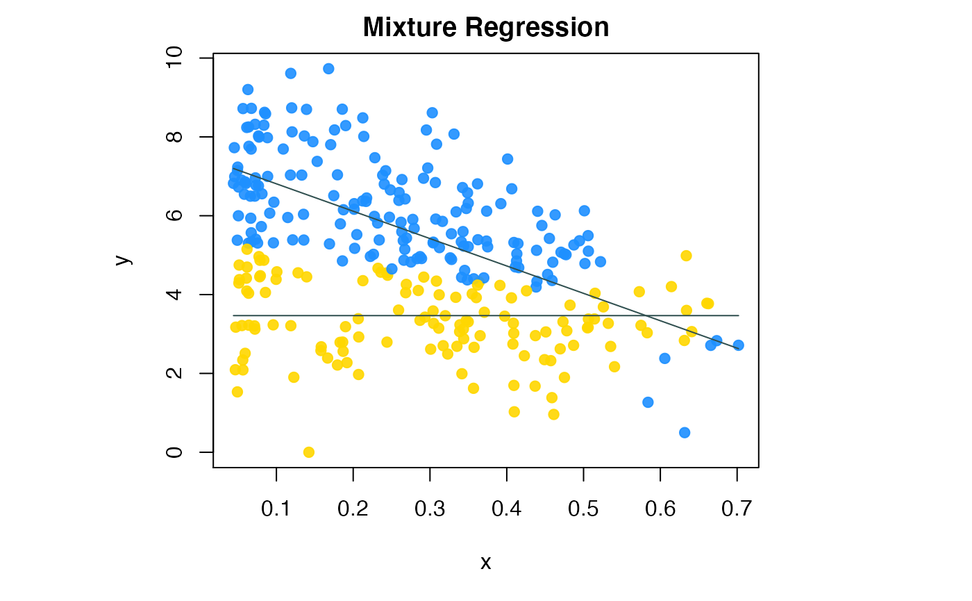
Colon cancer data flexible mixture regression
data(colon_data)
gene_expr = colon_data$x3
methylation = colon_data$y3
res.colon = MLM(ml.method="rmr", rmr.method='cat', x=gene_expr, y=methylation)
inds_in=which(res.colon$cluMem != -1)
par(mfrow=c(1,2),mar = c(4, 4, 6, 2))
compPlot(type='rlr', x=gene_expr,y=methylation,nc=2, inds_in=inds_in)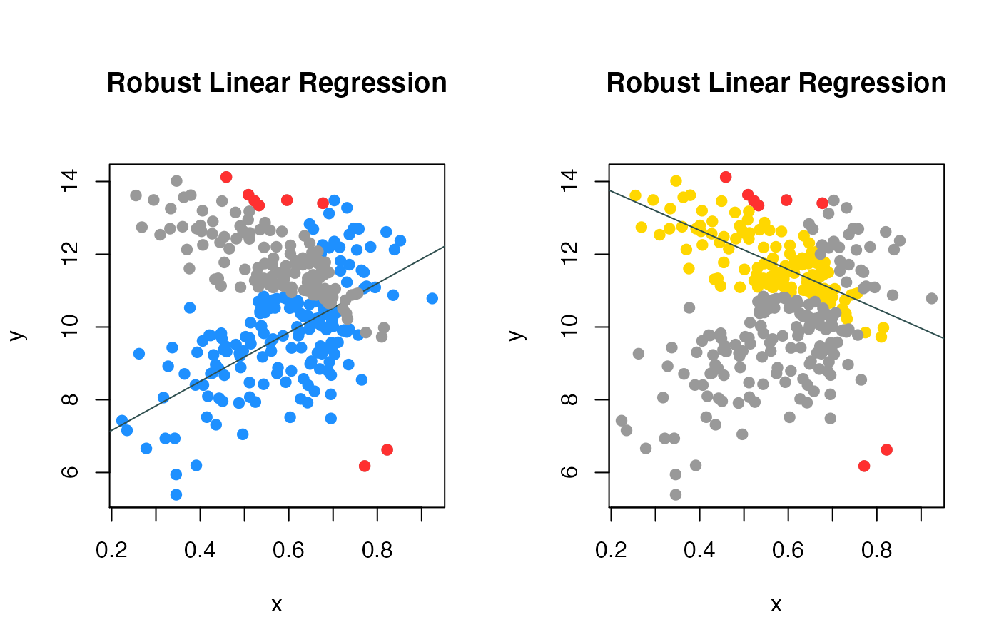
Colon cancer data robust mixture regression
We fitted the data using CAT, the two colored line represented the two subgroups of patients.
S3.2 Subspace clustering on high dimension dataset - CCLE application
We collected gene expression data of 470 cell lines as well as the cell lines’ sensitivity score (AUCC score) for ‘AEW541’ drug from the Cancer Cell Line Encyclopedia (CCLE) dataset. We demonstrate the usage of our package on this high dimensioanl dataset.
## [1] 490 500
rr = paste('row_', rownames(x), sep='')
cc = paste('col_', colnames(x), sep='')
rownames(x) = rr
colnames(x) = cc

y = CCLE_data$Y
y[is.na(y)] = 0
names(y) = rownames(x)

# suppress the output of warning informaiton
sink("nul") ; CCLE_res=MLM(ml.method="hrmr",x=x,y=y,nit=1,nc=2,max_iter=10); sink()
CCLE_coffs1=CCLE_res$coff

# plot the coefficient matrix
CCLE_res2 = list()
# just print rows (genes) whose coefficient is n
CCLE_res2$coff = CCLE_coffs1[which(apply(CCLE_coffs1,1,sum)!=0),]
compPlot(type='block', res=CCLE_res2)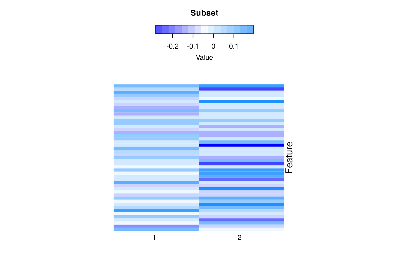
High dimension space feature robust mixture regression result